Number Sieves — Volume 4 — Congruences Made Mechanical

4.1 About This Volume

This volume is the mathematical hinge of the series. Volumes 2 and 3 described sieves that cross out multiples and, more generally, residue classes. Volumes 5 to 8 describe machines built from chains, gears, film and delay lines. Between the two sits a small body of arithmetic — congruences — that explains why a loop of 7 chain links can stand in for the number 7, why marking some of its links is the same as stating a condition on remainders, and why a set of such loops turning together will stop on exactly the numbers that satisfy every condition at once.

The volume builds that arithmetic in order: clock arithmetic and Gauss’s notation for it; residues and the rules for computing with them; which residues a perfect square can leave, and the Legendre symbol that records the answer; the Chinese Remainder Theorem, which guarantees that loops of coprime lengths act independently; Gauss’s “method of exclusion”; and Fermat’s method of factoring by a difference of squares. It then works one example completely, by hand and by machine: the factoring of 7663. Every number in that example has been checked by computer, and every step can be checked with a pencil. The volume ends by explaining why each well-chosen modulus throws away about half of the candidates, so that k moduli together leave roughly one in 2ᵏ.

4.2 Clock Arithmetic

At 9 o’clock, five hours later it is 2 o’clock, not 14. A clock face discards whole laps of 12 and keeps only the remainder. Arithmetic done this way — adding and multiplying as usual, then keeping only the remainder after division by a fixed number — is modular arithmetic, and the fixed number (12 on a clock) is the modulus.

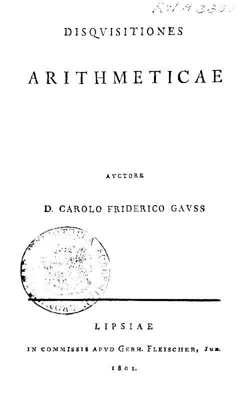
Carl Friedrich Gauss gave the subject its notation in his Disquisitiones Arithmeticae of 1801 (Wikisource translation). Two whole numbers a and b are congruent modulo m, written

a ≡ b (mod m),

when they leave the same remainder on division by m — equivalently, when their difference a − b is a multiple of m. So 14 ≡ 2 (mod 12), 9 ≡ 2 (mod 7), and 100 ≡ 0 (mod 5).

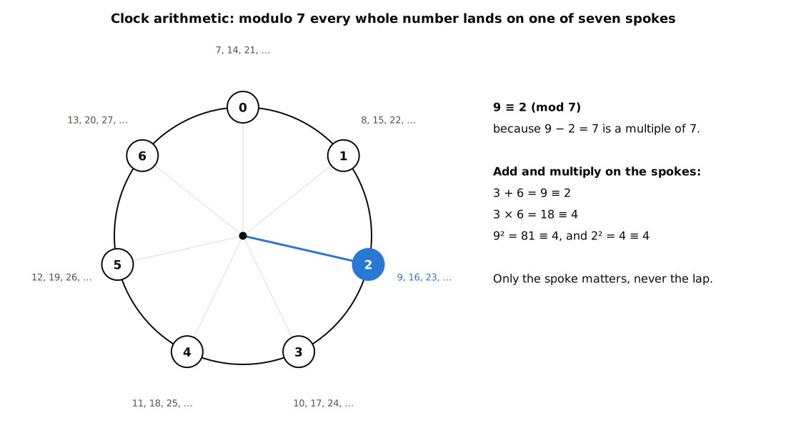
The remainder itself, a whole number from 0 to m − 1, is the residue of a modulo m, and the set of all numbers with the same residue — {…, −5, 2, 9, 16, 23, …} for residue 2 modulo 7 — is a residue class. Modulo m there are exactly m residue classes, one for each spoke of the clock.

4.2.1 The two rules that make it work

What makes modular arithmetic useful, rather than merely tidy, is that sums and products respect it. If a ≡ a′ and b ≡ b′ modulo m, then

• a + b ≡ a′ + b′ (mod m), and
• a × b ≡ a′ × b′ (mod m).

So to find the residue of a big expression, reduce each piece first and work with the small residues. Modulo 7, 3 + 6 = 9 ≡ 2, and 3 × 6 = 18 ≡ 4. Most important for this series, squares respect it too: 9 ≡ 2 (mod 7), so 9² ≡ 2² ≡ 4 (mod 7) — and indeed 81 = 11 × 7 + 4. The residue of b² modulo m depends only on the residue of b. That one fact is what lets a loop of m positions represent everything a sieve needs to know about b.

4.3 Which Remainders Can a Square Leave?

Square the numbers 0 to 4 and reduce modulo 5: 0, 1, 4, 9 ≡ 4, 16 ≡ 1. Only 0, 1 and 4 appear. No perfect square, however large, ever leaves remainder 2 or 3 on division by 5. The same experiment for every small modulus is shown in the figure.

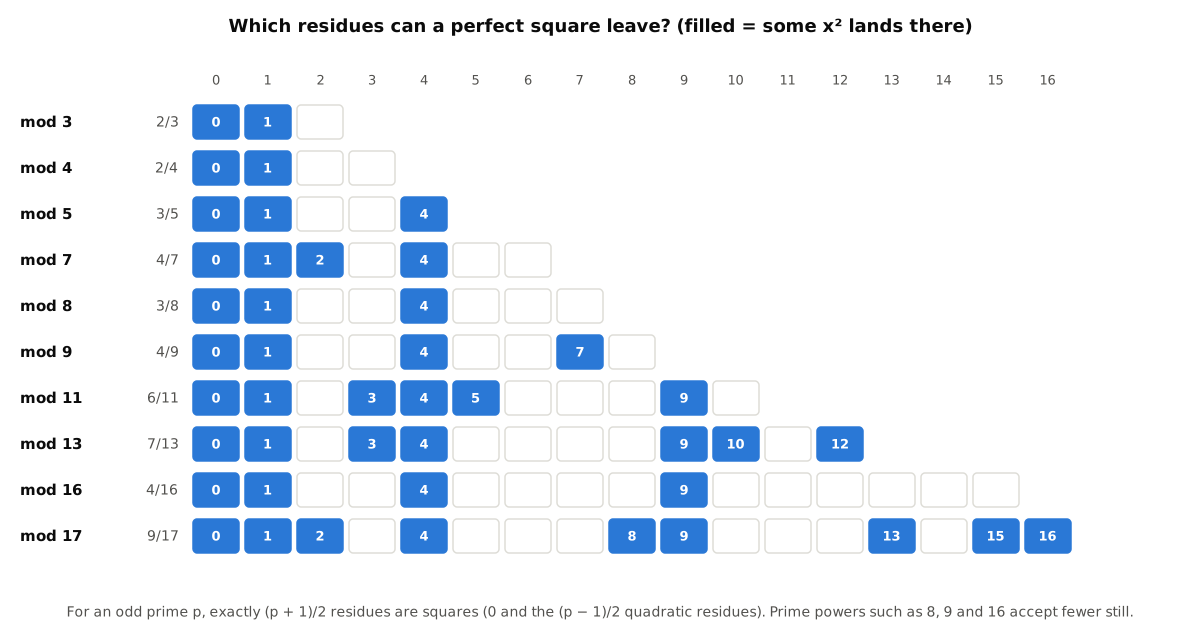
This gives a free, instant test that rejects most numbers as non-squares. A number ending in 2, 3, 7 or 8 is not a square (that is the test modulo 10). A number that leaves 2 or 3 on division by 5, or 3, 5 or 6 on division by 7, is not a square. Combining several such tests rules out the great majority of numbers without ever computing a square root.

4.3.1 Quadratic residues and the Legendre symbol

For an odd prime p, a residue a that is not 0 is called a quadratic residue modulo p if it is a square modulo p (some x has x² ≡ a), and a quadratic non-residue otherwise. Exactly half of the p − 1 non-zero residues are quadratic residues. The reason is that x and −x have the same square, so the p − 1 non-zero values of x pair off into (p − 1)/2 pairs, each pair giving one square, and no two pairs give the same square. Modulo 7, for example, 1² ≡ 6² ≡ 1, 2² ≡ 5² ≡ 4 and 3² ≡ 4² ≡ 2, so the quadratic residues are 1, 2 and 4, and the non-residues are 3, 5 and 6.

Adrien-Marie Legendre introduced a compact notation for this in 1798. The Legendre symbol (a/p) is

• +1 if a is a quadratic residue modulo p,
• −1 if a is a non-residue, and
• 0 if p divides a.

Leonhard Euler had already found a way to compute it: (a/p) ≡ a^((p−1)/2) (mod p) — Euler’s criterion. And the deepest fact about it, quadratic reciprocity, connects (p/q) with (q/p) for two odd primes p and q: they are equal unless both p and q leave remainder 3 on division by 4, in which case they are opposite. Euler and Legendre conjectured it; Gauss gave the first complete proof in 1796, at eighteen, and called it the theorema aureum, the golden theorem. Reciprocity is what lets a number theorist decide, for a given N, which primes make useful moduli without trying them all — a question that matters a great deal in choosing loops for a sieve machine.

4.4 The Chinese Remainder Theorem

Volume 1 solved a puzzle from the fifth-century Chinese Sunzi Suanjing by sieving: the number that leaves 2 on division by 3, 3 on division by 5 and 2 on division by 7 is 23. The general principle behind it is the Chinese Remainder Theorem (Wikipedia, “Chinese remainder theorem”):

If the moduli m₁, m₂, …, mₖ are pairwise coprime (no two share a common factor), then for any choice of residues r₁, r₂, …, rₖ there is exactly one number x between 0 and m₁ × m₂ × … × mₖ − 1 with x ≡ r₁ (mod m₁), x ≡ r₂ (mod m₂), …, x ≡ rₖ (mod mₖ).

Qin Jiushao gave a complete general method for solving such systems in his Mathematical Treatise in Nine Sections of 1247, and Gauss proved the theorem in the Disquisitiones with the modern notation.

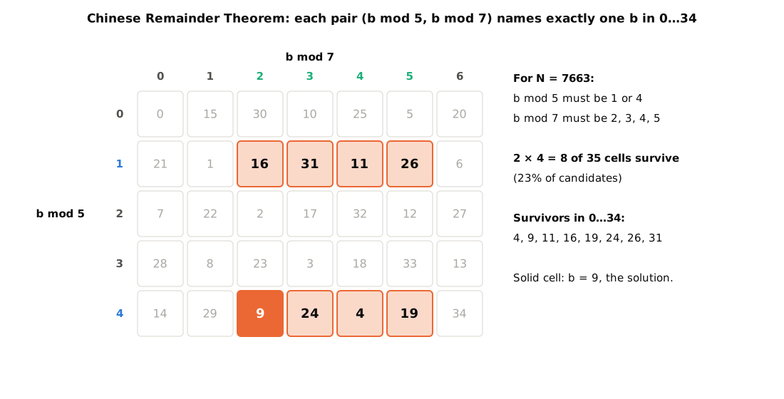
The theorem is easiest to see in a grid. Take the moduli 5 and 7, with product 35. Lay out a table with five rows (the residue modulo 5) and seven columns (the residue modulo 7), and write each number from 0 to 34 in the cell given by its two residues. Every one of the 35 cells receives exactly one number.

Two consequences matter for sieve machines.

Independence. Because every combination of residues occurs exactly once per period, a test modulo 5 and a test modulo 7 are independent: knowing a candidate passed one says nothing about whether it passes the other. If the modulo-5 test keeps 2 residues of 5 and the modulo-7 test keeps 4 of 7, then together they keep exactly 2 × 4 = 8 of every 35 numbers. Fractions of survivors multiply.

Period. A set of loops of lengths 5 and 7, all turning together, returns to its starting position only after 35 steps — the product of the lengths. A machine with many coprime loops has an enormous period: the nineteen prime moduli from 2 to 67 have a product of about 7.9 × 10²⁴, so the pattern of aligned tabs never repeats within any search a machine could run. Within that period, each combination of loop positions occurs exactly once.

Coprimality is essential. Loops of length 4 and 6 share the factor 2, so they realign every 12 steps, not every 24, and half of the 24 combinations of positions never occur at all. A tab at an even position on one loop can never meet a tab at an odd position on the other. That is why the Lehmers’ chains and gears used pairwise-coprime lengths: primes, and powers of distinct primes such as 16, 9, 25 and 49.

4.5 Gauss’s Method of Exclusion

In articles 319 to 322 of the Disquisitiones, Gauss describes a way to solve the congruence x² ≡ A by exclusion: for a series of small moduli E, called excludents, list the residues modulo E that are impossible, and strike out every candidate that falls on one of them (Wikisource translation; MathWorld, “Excludent factorization method”). He applied the same idea to factoring by a difference of squares. By hand the bookkeeping is naturally done with one strip of paper per excludent, the acceptable residues marked along it, the strips laid side by side so that a candidate’s column can be read across all of them.

That is a sieve machine in all but hardware. A Lehmer chain or gear is an excludent made of steel, and the moment of alignment that Gauss read by eye is the moment the Lehmers’ contacts close or their light beam gets through.

4.6 Fermat’s Method: Factoring by a Difference of Squares

4.6.1 The idea

Every odd number that has a factorisation N = u × v (with u ≤ v) can be written as a difference of two squares:

N = a² − b², with a = (u + v)/2 and b = (v − u)/2.

Conversely, if N = a² − b², then N = (a − b)(a + b), and unless a − b = 1 that is a genuine factorisation. Pierre de Fermat proposed factoring N by searching for such a and b: start with a equal to the smallest whole number whose square is at least N, and increase a one step at a time until a² − N is a perfect square b² (Wikipedia, “Fermat’s factorization method”).

A small example: N = 5959. The square root is about 77.2, so start with a = 78. Then 78² − 5959 = 125 (not a square), 79² − 5959 = 282 (not a square), 80² − 5959 = 441 = 21². So a = 80, b = 21 and 5959 = (80 − 21)(80 + 21) = 59 × 101.

In a 1643 letter to Marin Mersenne, Fermat used the method on 2,027,651,281. Its square root is about 45,029.4; starting from a = 45,030 and stepping upward, the twelfth trial, a = 45,041, gives a² − N = 1,040,400 = 1,020², so the number is (45,041 − 1,020)(45,041 + 1,020) = 44,021 × 46,061 (PrimePages, “2027651281”).

4.6.2 Why it needs a sieve

Fermat’s method is fast when the two factors are close together — then b is small and a starts very near the answer — and hopelessly slow when they are far apart, since a must climb from √N to (u + v)/2. Each trial also requires checking whether a number is a perfect square, which by hand is the slow part.

The residue facts above remove almost all of that work. Most candidates can be rejected because a² − N, or b² + N, leaves a remainder that no square can leave. Fermat already used the last digits for this. Gauss’s exclusion method formalised it. The Lehmers mechanised it: one loop per modulus, tabs on the residues of b for which b² + N could still be a square, and all loops turning together. Only the survivors need the expensive square-root check, and with enough moduli there are very few survivors.

4.7 The Worked Example: Factoring 7663

The example below follows the one in kbsriram’s A Tiny Sieve project, which uses it to explain the electronic sieve of Volume 8 (kbsriram, Hackaday.io). Every number has been checked.

4.7.1 Setting up the search

The task is to factor N = 7663. Instead of stepping through a, as Fermat did, search through b: find the smallest b ≥ 1 for which

b² + 7663 = a²

is a perfect square. Then 7663 = (a − b)(a + b).

Searching on b is convenient for a machine because b simply counts up 1, 2, 3, … — it is the number of steps the drive shaft has turned — and the test on each b is a statement about b’s residues. (For this particular N, Fermat’s own search on a happens to succeed at once, because the factors turn out to be close together; the example is chosen to show the sieve mechanics clearly, not to beat Fermat.) The search can be restricted to the range 1 ≤ b ≤ 3,831; at b = 3,831, (N − 1)/2, it reaches the trivial factorisation 1 × 7663.

4.7.2 The modulo-5 loop

First reduce N: 7663 = 5 × 1532 + 3, so 7663 ≡ 3 (mod 5). For each residue of b modulo 5, compute b² + 3 modulo 5 and ask whether the result is one of the square residues {0, 1, 4}:

Table 1 — First reduce N: 7663 = 5 × 1532 + 3, so 7663 ≡ 3 (mod 5). For each residue of b modulo 5, compute b² + 3 modulo 5 and ask whether the result is one of the square residues {0, 1, 4}

b mod 5	b² mod 5	b² + 7663 mod 5	Can it be a square?
0	0	3	no
1	1	4	yes
2	4	2	no
3	4	2	no
4	1	4	yes

So b must be ≡ 1 or 4 (mod 5). On a loop of 5 links, tabs go on positions 1 and 4. This loop alone throws away three-fifths of all candidates.

4.7.3 The modulo-7 loop

Next, 7663 = 7 × 1094 + 5, so 7663 ≡ 5 (mod 7). The square residues modulo 7 are {0, 1, 2, 4}.

Table 2 — The modulo-7 loop

b mod 7	b² mod 7	b² + 7663 mod 7	Can it be a square?
0	0	5	no
1	1	6	no
2	4	2	yes
3	2	0	yes
4	2	0	yes
5	4	2	yes
6	1	6	no

So b must be ≡ 2, 3, 4 or 5 (mod 7). On a loop of 7 links, tabs go on positions 2, 3, 4 and 5.

4.7.4 Running the two loops

Now turn both loops together, one position per step, starting from b = 0, and watch for the steps where both loops show a tab.

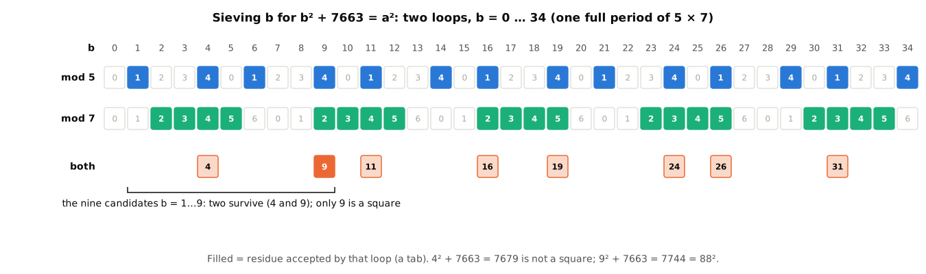
Table 3 — Running the two loops

b	b mod 5	tab on 5-loop?	b mod 7	tab on 7-loop?	Both?
1	1	yes	1	no	—
2	2	no	2	yes	—
3	3	no	3	yes	—
4	4	yes	4	yes	survivor
5	0	no	5	yes	—
6	1	yes	6	no	—
7	2	no	0	no	—
8	3	no	1	no	—
9	4	yes	2	yes	survivor

Of the nine candidates b = 1 to 9, the two loops reject seven and pass two: b = 4 and b = 9. These are the only ones that need the expensive check.

• b = 4: 4² + 7663 = 7679. Since 87² = 7569 and 88² = 7744, 7679 is not a perfect square. A false alarm: 7679 leaves acceptable remainders modulo 5 and 7, but it is not a square.
• b = 9: 9² + 7663 = 81 + 7663 = 7744 = 88². A perfect square.

So a = 88, b = 9, and

7663 = (88 − 9)(88 + 9) = 79 × 97.

Both 79 and 97 are prime, so the factorisation is complete.

4.7.5 Adding loops removes false alarms

The false alarm at b = 4 is exactly what more loops are for. Two more small moduli dispose of it:

• Modulo 3. 7663 ≡ 1 (mod 3), and the squares modulo 3 are {0, 1}. b² + 1 is 1 (a square residue) when b ≡ 0 and 2 (not a square residue) when b ≡ 1 or 2. So the modulo-3 loop has a single tab, at position 0: b must be a multiple of 3. That rejects b = 4.
• Modulo 8. 7663 ≡ 7 (mod 8), and squares modulo 8 are {0, 1, 4}. If b is odd, b² ≡ 1 and b² + 7 ≡ 0, a square residue; if b is even, b² + 7 is 7 or 3, neither of which is. So b must be odd — again rejecting b = 4.

With loops of 3, 5, 7 and 8 running together, b = 9 is the only survivor in the range 1 to 9: the machine stops once, on the answer. Run over the whole search range 1 to 3,831 with loops of 3, 5, 7, 8, 11 and 13, only 35 of the 3,831 candidates survive — under one percent — and the square-root check on those 35 finds exactly two genuine solutions: b = 9, giving 79 × 97, and b = 3,831, giving the trivial 1 × 7663.

4.8 Why a Loop with Tabs Is a Modulus

The example can now be read back as a description of a machine.

• A loop of m positions is the modulus m. Advance it one position per candidate and, after b steps, the position under the pointer is b mod m. The loop does not compute the residue; it embodies it, because both the loop and the residues repeat with period m.
• The tabs are the acceptable residue classes. A tab at position r says “candidates with b ≡ r (mod m) pass this test.” The list of tab positions on the 5-loop for N = 7663, {1, 4}, is precisely the right-hand column of the modulo-5 table above.
• A switch over the loop is the test. It closes when a tab passes under it — that is, when the current candidate’s residue is acceptable.
• Switches in series are the logical AND of all the tests. Current flows only when every switch is closed at once, so the circuit completes only for candidates acceptable to every modulus. The mirror image works equally well, and it is what Lehmer actually built in 1926–28: normally closed contacts in parallel, each opened by a tab, so the circuit breaks only when every loop shows a tab at once (Volume 6).
• Aligned tabs on all loops mean a candidate that survives every test. By the Chinese Remainder Theorem, each such alignment corresponds to exactly one value of b within the combined period, and the step counter on the drive shaft shows which.

The figure in Volume 1 shows the three loops for moduli 3, 5 and 7 at the moment b = 9, with all three tabs under their switches.

Changing the problem means moving tabs, not rebuilding the machine. To factor a different N, recompute N modulo each loop length, recompute which residues of b are acceptable, and reset the tabs. On a chain the tab is a pin or long-tailed screw fitted at a chosen link, and it can be moved to another link; Volumes 6, 7, 11 and 12 describe how each machine was (or can be) re-set. The loop lengths are fixed; the tab pattern is the program.

Two refinements, both covered in the build volumes, follow from the arithmetic.

• Prime-power loops are stronger than prime loops. A loop of 8 positions rejects more than a loop of 2, and a loop of 9 more than a loop of 3, because squares are more constrained modulo prime powers (only 0, 1 and 4 modulo 8; only 0, 1, 4 and 7 modulo 9). The first gears of Lehmer’s 1932 gear sieve had prime-power tooth counts for this reason (kbsriram).
• The loop lengths must be pairwise coprime, or some combinations of tab positions can never line up and the machine silently skips candidates.

4.9 Why k Moduli Leave About One Candidate in 2ᵏ

For N = 7663 the modulo-5 loop kept 2 of 5 residues, and the modulo-7 loop kept 4 of 7. Neither is exactly half, but both are close, and that is no accident.

For an odd prime p that does not divide N, count the residues b modulo p for which b² + N is a square residue (including 0). The answer is always

(p + (−N/p)) / 2,

where (−N/p) is the Legendre symbol of −N: that is, (p + 1)/2 if −N is a quadratic residue modulo p, and (p − 1)/2 if it is not. For p = 5, −7663 ≡ 2, a non-residue modulo 5, giving (5 − 1)/2 = 2 acceptable residues. For p = 7, −7663 ≡ 2, a residue modulo 7, giving (7 + 1)/2 = 4. (A sketch of why: the equation a² − b² ≡ N has exactly p − 1 solutions (a, b) modulo p; each acceptable b with b² + N ≢ 0 contributes two values of a, and each with b² + N ≡ 0 contributes one, and counting gives the formula.)

So each prime modulus keeps very nearly half of the candidates, and by the Chinese Remainder Theorem the moduli act independently, so their fractions multiply. With k prime moduli the survivors are roughly

(1/2) × (1/2) × … × (1/2) = 1/2ᵏ

of the candidates. For N = 7663 and the eighteen odd primes from 3 to 67, the exact product of the fractions is about 1 in 429,000 (against 1 in 2¹⁸ ≈ 262,000; the moduli 3 and 5 keep well under half). Add a modulus of 8 or 16 for the prime 2 and the figure falls further.

This is the arithmetic behind every claim of sieve-machine power in the later volumes. Lehmer’s 1926 chains, with links counted to the nineteen primes up to 67, let through roughly one candidate in half a million; his photoelectric gear sieve of 1932, with 30 gears, roughly one in a billion. A survivor is not yet an answer — b = 4 above shows that — but with that many moduli the survivors are so rare that checking each one by hand is no burden, and the expensive part of the work has been done by nothing more than turning a shaft.

4.10 Summary

• Modular arithmetic keeps only remainders; sums, products and squares can all be computed on residues alone.
• A perfect square can occupy only about half the residues modulo any odd prime; prime powers constrain it further. The Legendre symbol records which.
• For pairwise coprime moduli the Chinese Remainder Theorem makes the tests independent: survivor fractions multiply, and the combined pattern repeats only after the product of the moduli.
• Fermat’s difference-of-squares method turns factoring into a search for a square; Gauss’s exclusion method turns that search into a sieve on residues.
• A loop of m positions with tabs on the acceptable residues is a modulus with its acceptable classes; switches in series are the logical AND; aligned tabs mark the survivors.
• Each prime modulus keeps about half the candidates, so k moduli keep about one in 2ᵏ.

The example of 7663 needed two loops and nine steps. The Lehmers’ problems needed twenty or thirty loops and millions of steps — which is where the machines begin.

---

Next — Volume 5: Before the Machines. The people who first tried to turn exclusion into machinery: F. W. Lawrence’s 1896 design, André Gérardin and Maurice Kraitchik in Paris, Eugène-Olivier Carissan’s hand-cranked machine à congruences of 1919 and its rediscovery in a Bordeaux drawer seventy years later — and the Berkeley family, Derrick Norman and Derrick Henry Lehmer and Emma Lehmer, who made sieve machines a life’s work.