Number Sieves — Volume 3 — Beyond Eratosthenes: Wheels, Segments and Sieve Theory

3.1 About This Volume

Volume 2 ran the Sieve of Eratosthenes as Nicomachus described it, with a few modern efficiencies. This volume follows the sieve in two directions at once.

The first direction is practical: how to make the sieve fast and small. Wheel factorisation skips the multiples of the first few primes before sieving starts; the segmented sieve processes a huge range one cache-sized window at a time; Euler’s sieve, the Sieve of Sundaram and the Sieve of Atkin rearrange the work in different ways. A short Python listing shows the plain and segmented sieves in a couple of dozen lines, and the section on records describes the programs that count and list primes into the quintillions.

The second direction is theoretical: what can be proved by thinking about what a sieve leaves behind, without running it. Legendre turned the sieve into a counting formula; Viggo Brun turned it into a tool sharp enough to show that the twin primes are sparse; Atle Selberg and the “large sieve” of Linnik, Rényi, Roth and Bombieri turned it into one of the central machines of modern analytic number theory, the engine inside Zhang’s and Maynard’s theorems on prime gaps.

The volume ends with the idea that connects both directions to the rest of the series: a sieve does not have to cross out multiples. It can cross out any residue class — every number that leaves a particular remainder on division by m. That is what the Lehmers’ chains and gears do.

3.2 Wheel Factorisation: Sieving Only What Could Be Prime

Nicomachus already knew the first trick: the even numbers (after 2) are composite, so there is no point writing them down. Sieving only the odd numbers halves the memory and removes the most expensive pass — the one for 2 — entirely.

The idea generalises. After 2 and 3, every prime leaves remainder 1 or 5 on division by 6, because a number that leaves 0, 2 or 4 is even and one that leaves 3 is divisible by 3. So only two numbers in every six need to be considered: a third of the original list. After 2, 3 and 5 together, only the eight residues 1, 7, 11, 13, 17, 19, 23 and 29 modulo 30 can hold a prime — 8 numbers in every 30, or about 27 percent.

Arranged in a circle, these allowed residues look like the spokes of a wheel, which gives the method its name. A sieve built on the 30-wheel lays out its numbers in blocks of 30, keeps one bit for each of the 8 spokes in each block, and steps through them using the fixed gaps between spokes (6, 4, 2, 4, 2, 4, 6, 2, and round again). A convenient coincidence makes the 30-wheel especially popular in software: eight spokes per block fit exactly into one byte.

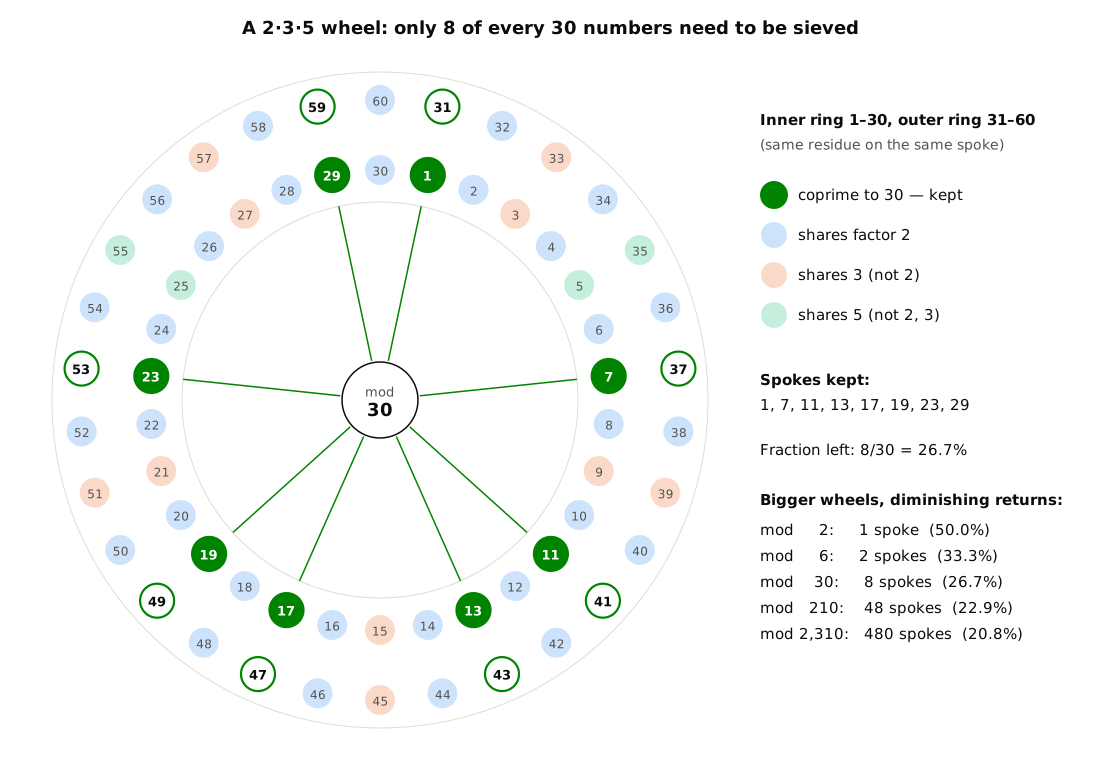
Bigger wheels give diminishing returns. The fraction of numbers a wheel keeps is the product (1 − 1/2)(1 − 1/3)(1 − 1/5)…, over the primes in the wheel: one-half, one-third, 8/30, 48/210, 480/2,310. That product shrinks only like 1/ln of the largest prime involved — a fact due to Mertens, and the same fact that gave the sieve its N log log N running time in Volume 2. Past the 30- or 210-wheel, the extra bookkeeping usually costs more than it saves. Paul Pritchard used wheels that grow with N to build sieves whose operation count is proportional to N alone, without the log log N factor, in a series of papers in the early 1980s; in practice a well-tuned segmented sieve with a modest fixed wheel is faster (Wikipedia, “Sieve of Eratosthenes”).

A wheel is a sieve’s first encounter with residue classes. Rejecting “everything that leaves 0, 2, 3, 4, 5, 6, 8, 9, 10, … on division by 30” is a statement about remainders, not multiples, and the wheel can be imagined as a physical loop of 30 positions with eight of them marked. That is precisely the kind of loop the Lehmers would build.

3.3 The Segmented Sieve: A Window onto Infinity

The basic sieve needs one mark per number. To list the primes up to 10¹², that is a trillion marks — more memory than most computers have, and far more than fits in a processor’s fast cache, where the crossing-out loop would like to run. The segmented sieve removes the problem.

The idea is the one used by hand in Volume 2’s exercise on 101–200. Since only the primes up to √N are needed to sieve to N, first find those base primes with an ordinary small sieve. Then process the range in consecutive segments (windows) of fixed size. For each window, and for each base prime p, compute the first multiple of p inside the window and cross out from there in steps of p. When the window is finished, report its survivors, then move on to the next window, carrying each prime’s position forward.

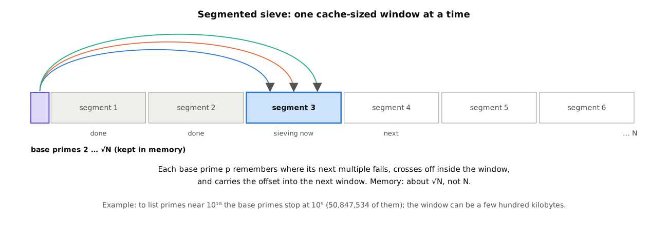
Memory now falls to about √N for the base primes plus one window. To list primes near 10¹⁸, the base primes stop at 10⁹ — there are 50,847,534 of them — and the window can be a few hundred kilobytes, sized to fit in the processor’s cache. The method was formalised by Carter Bays and Richard Hudson in 1977 (Wikipedia, “Sieve of Eratosthenes”).

A segmented sieve can start anywhere: to examine the million numbers just above 10¹⁸ there is no need to look at anything below them. That makes it the natural tool for record computations. Tomás Oliveira e Silva, Siegfried Herzog and Silvio Pardi used a highly optimised segmented sieve to verify the even Goldbach conjecture — that every even number greater than 2 is the sum of two primes — for every even number up to 4 × 10¹⁸, and to tabulate all prime gaps up to the same bound (Oliveira e Silva, Herzog & Pardi, Mathematics of Computation 83 (2014)). For primes much bigger than √(window), most primes skip over a window without touching it; their technique of keeping such primes in “buckets” sorted by the window they will next hit avoids looking at them at all until needed.

3.4 Other Ways to Cross Out

3.4.1 Euler’s sieve: every composite crossed out exactly once

In the Sieve of Eratosthenes, 30 is crossed out three times — once each by 2, 3 and 5. Euler’s sieve arranges the work so that each composite is removed exactly once, by its smallest prime factor: for each number k and each prime p up to the smallest prime factor of k, it crosses out p × k. The total work is proportional to N, rather than N log log N. David Gries and Jayadev Misra rediscovered the method as a “linear sieve” in 1978. In practice the bookkeeping is heavier than the few extra crossings it saves, and segmented Eratosthenes remains faster.

3.4.2 The Sieve of Sundaram

In 1934 S. P. Sundaram, then a student in India, published a sieve that never mentions primes at all (Wikipedia, “Sieve of Sundaram”). Start with the numbers 1 to n. Strike out every number of the form

i + j + 2ij, with 1 ≤ i ≤ j.

Then double each survivor and add 1. The results are exactly the odd primes up to 2n + 1.

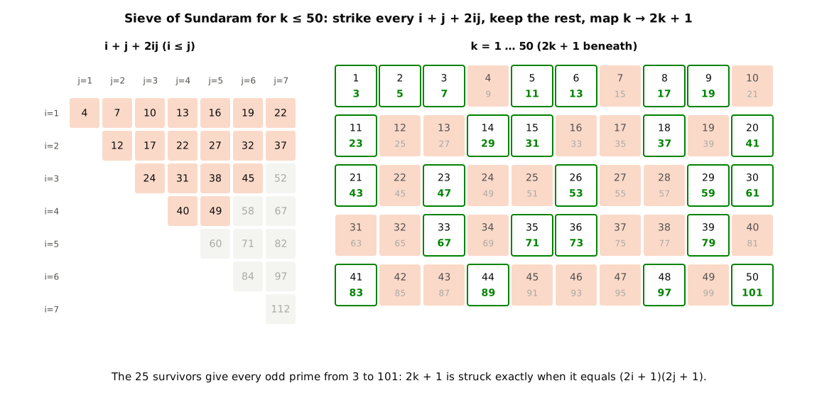
The reason it works is a short piece of algebra. If k = i + j + 2ij, then 2k + 1 = 2i + 2j + 4ij + 1 = (2i + 1)(2j + 1), a product of two odd numbers each at least 3. Conversely every odd composite can be written that way. So k is struck exactly when 2k + 1 is an odd composite, and the survivors map onto the odd primes. Sundaram’s sieve is, underneath, the odd-numbers-only Sieve of Eratosthenes written in disguise — and, like Nicomachus’ version, it wastes effort by crossing out with every odd factor rather than only the primes, so it runs in about n log n steps rather than n log log n. Its charm is that it can be done with a multiplication table and no knowledge of primes.

3.4.3 The Sieve of Atkin

In 2003 A. O. L. Atkin and Daniel J. Bernstein published a sieve that throws away the crossing-out of multiples altogether and replaces it with quadratic forms (Atkin & Bernstein, “Prime sieves using binary quadratic forms,” Mathematics of Computation 73 (2004)). It relies on classical results about which numbers can be written as 4x² + y², 3x² + y² or 3x² − y²: for a square-free n in the right residue classes modulo 60, n is prime exactly when the relevant form has an odd number of representations. The algorithm walks the lattice of (x, y) pairs, toggles a bit for each n it reaches, and finally removes multiples of squares (Wikipedia, “Sieve of Atkin”).

Table 1 — The Sieve of Atkin

n mod 60	Form whose representations are counted
1, 13, 17, 29, 37, 41, 49, 53	4x² + y² = n
7, 19, 31, 43	3x² + y² = n
11, 23, 47, 59	3x² − y² = n (with x > y)

In theory the Sieve of Atkin needs about N operations, fewer than Eratosthenes’ N log log N. In practice, the operations are more expensive and the memory access pattern less friendly, and the best segmented, wheel-factorised Sieve of Eratosthenes implementations are faster over every range anyone actually sieves. Bernstein released an optimised implementation, primegen; the fastest general-purpose prime generators in use today, such as primesieve (below), are nonetheless segmented Sieves of Eratosthenes.

3.5 Sieving in Code

A sieve is one of the few serious algorithms that fits in a few lines. Here is the plain sieve and a segmented version in Python. Both run on any Python 3 installation with no libraries.

from math import isqrt

def simple_sieve(n):
    """All primes <= n by the Sieve of Eratosthenes."""
    is_prime = bytearray([1]) * (n + 1)
    is_prime[0:2] = b"\x00\x00"
    for p in range(2, isqrt(n) + 1):
        if is_prime[p]:
            # cross out p*p, p*p+p, ... in one slice assignment
            is_prime[p*p::p] = bytes(len(range(p*p, n + 1, p)))
    return [i for i, flag in enumerate(is_prime) if flag]

def segmented_sieve(lo, hi, size=32768):
    """Primes in [lo, hi), one window of `size` numbers at a time."""
    base = simple_sieve(isqrt(hi - 1) + 1)          # primes up to sqrt(hi)
    for start in range(lo, hi, size):
        stop = min(start + size, hi)
        window = bytearray([1]) * (stop - start)
        for p in base:
            first = max(p * p, -(-start // p) * p)    # first multiple of p >= start, never below p*p
            window[first - start::p] = bytes(len(range(first, stop, p)))
        for i, flag in enumerate(window):
            if flag and start + i >= 2:
                yield start + i

print(simple_sieve(100))                     # the 25 primes below 100
print(list(segmented_sieve(101, 201)))       # the 21 primes from Volume 2's exercise
print(sum(1 for _ in segmented_sieve(10**9, 10**9 + 10**6)))   # 48155

The lines to notice:

• is_prime[p*p::p] = … is the whole of the sieve. Python’s slice assignment crosses out every p-th entry from p² onward in one operation — the “start at p²” rule from Volume 2, verbatim.
• range(2, isqrt(n) + 1) is the “stop at √N” rule.
• -(-start // p) * p is the hand calculation from Volume 2’s exercise: the first multiple of p at or above the window’s start. Wrapping it in max(p * p, …) keeps a base prime from crossing itself out when a window begins below its square.
• The last line sieves the million numbers just above one billion without ever touching the billion numbers below them, using only the 3,402 base primes up to √(10⁹ + 10⁶) ≈ 31,639. It finds 48,155 primes — about one in 20.8, close to the prime number theorem’s prediction of one in ln(10⁹) ≈ 20.7.

3.5.1 Record tables and the programs that make them

Hand-made prime tables reached their peak with D. N. Lehmer’s List of Prime Numbers from 1 to 10,006,721 (1914). Today the standard tool is Kim Walisch’s primesieve, an open-source C++ library that “generates primes using the segmented sieve of Eratosthenes with wheel factorization,” with O(√N) memory, a bucket sieve for large primes and support up to 2⁶⁴ (github.com/kimwalisch/primesieve).

Counting primes far beyond what can be listed needs a different approach. Legendre’s formula and its descendants (next section) compute π(x) without listing the primes. Ernst Meissel used such a method in the 1870s and 1880s to compute π(10⁸) by hand; D. H. Lehmer extended and simplified it in 1959 and, on an IBM 701, computed π(10⁹) correctly and π(10¹⁰) to within 1. Refinements by Lagarias, Miller and Odlyzko (1985), Deléglise and Rivat (1996) and Xavier Gourdon led to Walisch’s primecount, with which David Baugh and Walisch announced π(10²⁷) in 2015, π(10²⁸) in 2020 and π(10²⁹) in 2022 (Wikipedia, “Prime-counting function”). The last of these, 1,520,698,109,714,272,166,094,258,063, is the current record (OEIS A006880).

Jonathan Sorenson’s An Introduction to Prime Number Sieves (University of Wisconsin technical report 909, 1990) remains a clear survey of the algorithms in this section and their costs (PDF).

3.6 Legendre: Counting Survivors Without Running the Sieve

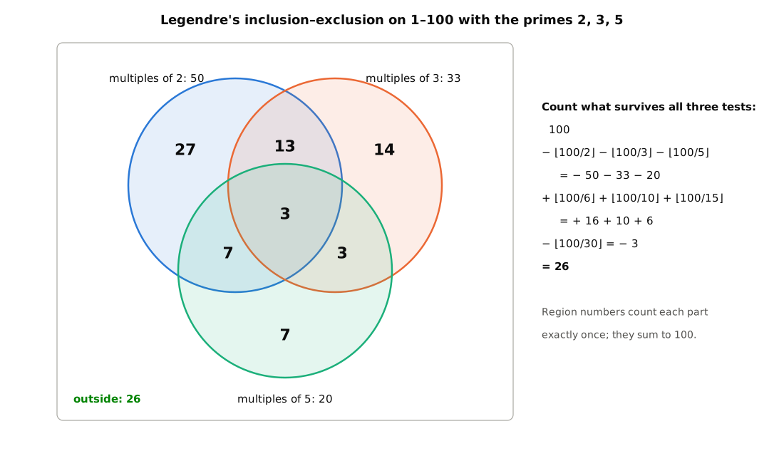
The rest of this volume is about sieve theory: the mathematics of estimating how many numbers survive a sieve. It begins with a simple question. Sieve the numbers 1 to 100 by the primes 2, 3 and 5. How many survive?

Count the casualties. 50 numbers are multiples of 2, 33 of 3 and 20 of 5 — but subtracting all of those removes the multiples of 6, 10 and 15 twice, so add back 16, 10 and 6; and that in turn adds back the multiples of 30 once too often, so subtract 3. The answer is

100 − 50 − 33 − 20 + 16 + 10 + 6 − 3 = 26.

This is the inclusion–exclusion principle, and the numbers in each step are just whole parts of divisions: ⌊100/2⌋ = 50, ⌊100/6⌋ = 16, and so on.

Adrien-Marie Legendre made this into a formula for the number of primes. Sieving 1 to x by the primes up to √x leaves 1 and the primes between √x and x; so if φ(x, a) is the number of integers up to x not divisible by any of the first a primes, then

π(x) = φ(x, a) + a − 1, where a = π(√x).

For x = 100, a = 4 (the primes 2, 3, 5, 7), φ(100, 4) = 22 and π(100) = 22 + 4 − 1 = 25. And φ itself can be computed by inclusion–exclusion: a signed sum of ⌊x/d⌋ over all products d of distinct primes from the list.

Legendre’s formula is exact, and it is the ancestor of every modern prime-counting algorithm. It has two weaknesses, and the history of sieve theory is largely the history of working around them.

• Too many terms. With a primes in the list there are 2ᵃ products d to sum over. For x = 10⁶ there are 168 primes below √x and 2¹⁶⁸ terms. Meissel’s and Lehmer’s methods, and their successors, reorganise the sum to avoid most of them.
• Too much rounding. As an estimate, inclusion–exclusion wants to replace ⌊x/d⌋ by x/d and so get x times the product (1 − 1/2)(1 − 1/3)(1 − 1/5)…. But each of the 2ᵃ terms carries a rounding error of up to 1, and with exponentially many terms the errors swamp the answer. Legendre’s sieve, used as an approximation, proves almost nothing.

3.7 Brun’s Sieve and the Twin Primes

The Norwegian mathematician Viggo Brun found the way round the second problem in 1915. His insight was that inclusion–exclusion does not have to be carried to the end. Stop the alternating sum after an even number of steps and the partial result is an upper bound for the true count; stop after an odd number and it is a lower bound. Truncate cleverly — keeping only the terms where d has a limited number of prime factors — and the number of terms, and with them the rounding errors, stays under control, while the bounds remain close enough to be useful. Brun’s 1915 paper on Goldbach’s problem is where the word “sieve” first entered number theory as a technical term (Wikipedia, “Sieve theory”).

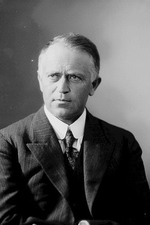
Brun applied the sieve to two classic problems (Wikipedia, “Brun sieve”).

Twin primes. To find twin primes, sieve the numbers n so that both n and n + 2 survive: for each small prime p, cross out the residue class n ≡ 0 (mod p) and the class n ≡ −2 (mod p). That is the first sieve in this series that removes two residue classes per prime instead of one — and it is a sieve of exactly the kind the Lehmers’ machines run. Brun’s method showed that the number of twin primes up to x is at most a constant times x (log log x)² / (log x)², which is smaller than the count of primes by nearly a whole factor of log x. It follows that the sum of the reciprocals of the twin primes,

(1/3 + 1/5) + (1/5 + 1/7) + (1/11 + 1/13) + (1/17 + 1/19) + …,

converges to a finite number, even though the sum of the reciprocals of all the primes grows without limit (Wikipedia, “Brun’s theorem”). The limit is Brun’s constant, B₂ ≈ 1.902160583104, an estimate by Pascal Sebah and Patrick Demichel (2002) from all the twin primes up to 10¹⁶. The convergence is excruciatingly slow: the partial sum over the twin primes below a million is only about 1.7108.

Brun’s theorem does not settle whether there are infinitely many twin primes — a convergent sum can have infinitely many terms — and that question remains open.

Goldbach. Brun’s sieve showed that every sufficiently large even number is the sum of two numbers each having at most nine prime factors. The “nine” was steadily whittled down by later sieve theorists, until in 1973 Chen Jingrun proved that every sufficiently large even number is the sum of a prime and a number with at most two prime factors — the closest anyone has come to Goldbach’s conjecture. The same method shows that there are infinitely many primes p for which p + 2 is either prime or the product of two primes.

3.7.1 The constant that found a bug

The heuristic count of twin primes, conjectured by G. H. Hardy and J. E. Littlewood in 1923, is

π₂(x) ≈ 2C₂ x / (ln x)², with the twin prime constant C₂ = ∏ over odd primes p of p(p − 2)/(p − 1)² ≈ 0.6601618158.

The constant is a sieve calculation in disguise: each factor p(p − 2)/(p − 1)² compares the fraction of pairs (n, n + 2) that survive the prime p (which removes two residue classes, leaving p − 2 of p) with what two independent random numbers would do. Below a million the simple formula predicts about 6,900 twin pairs against the true 8,169; the integral form 2C₂ ∫ dt / (ln t)² predicts about 8,250 — within one percent.

In 1994 Thomas Nicely of Lynchburg College was computing twin primes into the trillions to estimate Brun’s constant, running the same calculation on several machines as a check. The results from a new Intel Pentium disagreed with the others. Nicely traced the discrepancy to a flaw in the Pentium’s floating-point division unit — the “FDIV bug” — and the resulting public argument forced Intel into a costly recall (Wikipedia, “Brun’s theorem”).

3.8 Selberg’s Sieve and the Large Sieve, in Plain Words

3.8.1 Selberg: optimise the weights

Brun’s method decides which terms of inclusion–exclusion to keep by a fixed rule. In 1947 the Norwegian Atle Selberg asked a different question: if the inclusion–exclusion coefficients (the +1s and −1s) are replaced by adjustable weights, which choice of weights gives the best possible upper bound? Because his bound is a sum of squares, it can never go negative, and the optimal weights can be found by minimising a quadratic expression — essentially a least-squares problem (Wikipedia, “Selberg sieve”). The Selberg sieve gives clean, strong upper bounds with less effort than Brun’s and is a workhorse of modern number theory; a classic application is the Brun–Titchmarsh theorem, which bounds the number of primes in an arithmetic progression.

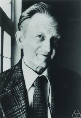
Selberg also identified the fundamental limitation of sieve methods, now called the parity problem: a sieve that only knows how many survivors fall in each residue class cannot, on its own, tell numbers with an odd number of prime factors from those with an even number. That is why sieve methods prove “a prime or a product of two primes” (Chen) but stall short of “a prime” (Goldbach, twin primes). Zhang’s 2013 theorem on bounded gaps, and Maynard’s refinement, used Selberg-type weights in a sieve devised by Goldston, Pintz and Yıldırım, and got round the parity barrier by asking for some pair among several candidates to be prime rather than a specific one.

3.8.2 The large sieve: when most classes are removed

The sieves so far remove only a few residue classes per prime: one for Eratosthenes, two for Brun’s twin primes. In 1941 Yuri Linnik, studying the smallest number that is not a perfect square modulo a prime, needed the opposite: a sieve that removes a large fraction — up to about half — of the residue classes modulo every prime (Wikipedia, “Large sieve”). The question the large sieve answers is: if a set of whole numbers up to N avoids many residue classes modulo every prime, how big can that set possibly be? The answer is “not very” — forbidding many classes for every prime squeezes the set hard. Alfréd Rényi developed the idea probabilistically; Klaus Roth and Enrico Bombieri gave it its definitive form in the 1960s, and Bombieri used it to prove the Bombieri–Vinogradov theorem, which says that primes are well distributed among residue classes “on average” and is one of the key ingredients in the bounded-gap theorems.

The large sieve matters to this series because its setting — remove roughly half of the residues modulo each of many moduli, and see what survives — is exactly the setting of the Lehmers’ factoring machines. A number that is a perfect square can only fall in about half of the residue classes modulo each prime, so a search for squares removes about half of all candidates at every modulus. Volume 4 shows this with the factoring of 7663, and it is why a sieve machine with twenty or thirty moduli is so effective. Linnik’s question about squares and Lehmer’s bicycle chains are two views of the same object.

3.9 From Multiples to Residue Classes

Step back and look at what has changed since Eratosthenes.

The original sieve removes, for each prime p, one residue class: the numbers that leave remainder 0 on division by p, which are the multiples of p. The wheel removes every residue class modulo 30 that shares a factor with 30. Brun’s twin-prime sieve removes two classes per prime, 0 and −2. The large sieve and the quadratic-residue sieves of the next volume remove about half the classes per modulus.

In every case the operation is the same: for each modulus m, decide which remainders are forbidden, and discard every candidate whose remainder modulo m is forbidden. The candidates that survive all the moduli are the answer. Crossing out multiples is merely the special case in which the forbidden remainder is 0.

That generalisation is what makes a sieve machine possible, because a residue class has a perfectly regular physical form. The numbers with remainder r modulo m recur every m steps, forever, so they can be represented by a mark at position r on a loop of length m. Eratosthenes needed a fresh stride for each prime and a written list to stride along. The Lehmers needed only a set of loops, one per modulus, each marked at its acceptable positions, all turning together — and no list at all. The candidates are simply the steps of the drive shaft, and the survivors are the moments when every loop shows a mark at once.

---

Next — Volume 4: Congruences Made Mechanical. The mathematics of the loop: clock arithmetic, residues and the notation Gauss invented for them, quadratic residues and the Legendre symbol, the Chinese Remainder Theorem, and Fermat’s difference-of-squares method — ending with the complete factoring of 7663 by two loops of chain, step by step, and the reason k well-chosen moduli cut the candidates to about one in 2ᵏ.